Third Tutorial: Complexity and Cellular Automata.
Cellular Automata.
This tutorial will look at one of the basic models used to represent complexity, known as Cellular Automata or CA for short. CAs were proposed by John von Neumann and Stanislaw Ulam in the late forties, while working at Los Alamos National Laboratory on the American nuclear program. CAs consist of a number of cells which can have different states, and certain rules for changing these, depending of the states of their neighbours. Through this very simple mechanism they can model a large number of natural phenomena, from fluid dynamics to the growth of corals or population dynamics and ecological systems. In 2002, Stephen Wolfram published his book “a New Kind of Science” , in which he proposed Cellular Automata and other simple computational models as the basis for a new way of representing, modelling and studying physical phenomena. Cellular Automata have also been proposed as models of city growth, and particularly studied by Michael Batty at UCL, together with other models of self-organisation.
In this tutorial we are going to look to how to write Cellular Automata in Processing. There are also a few examples accessible in the Examples folder (“File->Examples…”), under “Topics”(the examples are also available online at the Processing website). Some of these examples don’t follow the typical implementation of a CA. Also, there are a number of downloadable Processing code examples about complexity, including CAs, from Daniel Shiffman’s book “The Nature of Code“.
Basic concepts for implementing Cellular Automata.
Two dimensional arrays:
The previous tutorial looked at arrays; these consisted of a number of variables or objects accessible through the name of the array and an index, given between square brackets []. These arrays can be considered as one dimensional; one can imagine how the different elements in the array are arranged one after the other in a long row of some length, effectively of one dimension. But it is possible to arrange and access the elements in a different, sometimes more convenient, way; the example given here is for 2 dimensions, by the same principle ca be extended to 3 or even more dimensions.
A two dimensional array is not that different from a regular (one dimensional) array: instead of having one index, it has two:
SomeTwoDimensionalArray[index1][index2];
One can think of this 2 dimensional array as a table, a matrix or a grid organised in rows and columns. Here is a basic example that creates a 2 dimensional array, sets and the values of all elements in the array thorough a nested for loop (nested loops are the standard way of iterating through all elements of the array), sets also the value of one of the elements, and draws the values as the colours of rectangles on the screen:
size(400,400);
int numColumns=20, numRows=20;
int[][] a2DArray;

a2DArray=new int[numColumns][numRows];

//make all elements 255, we are going to use this as their colour.
//we need a nested loop for this:
for(int i=0;i<numColumns;i++){
 for(int j=0;j<numRows;j++){
  a2DArray[i][j]=255;
 }
}

//now we set the one in the middle black, for example
a2DArray[numColumns/2][numRows/2]=0;

//we also calculate a size for the "cells" in the array, depending
//of how many there are and the size of the screen.
int rectW=width/numColumns;
int rectH=height/numRows;

//and we draw all of them
for(int i=0;i<numColumns;i++){
 for(int j=0;j<numRows;j++){
  fill(a2DArray[i][j]);
  rect(i*rectW, j*rectH, rectW,rectH);
 }
}
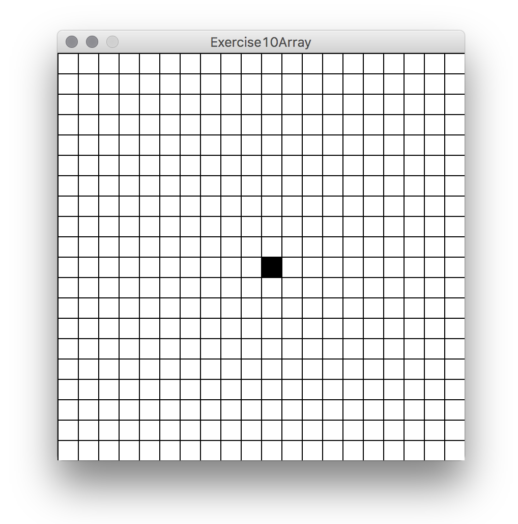
Here is a tutorial from the Processing website , if you want to learn more about 2 dimensional arrays.
Neighbourhood:
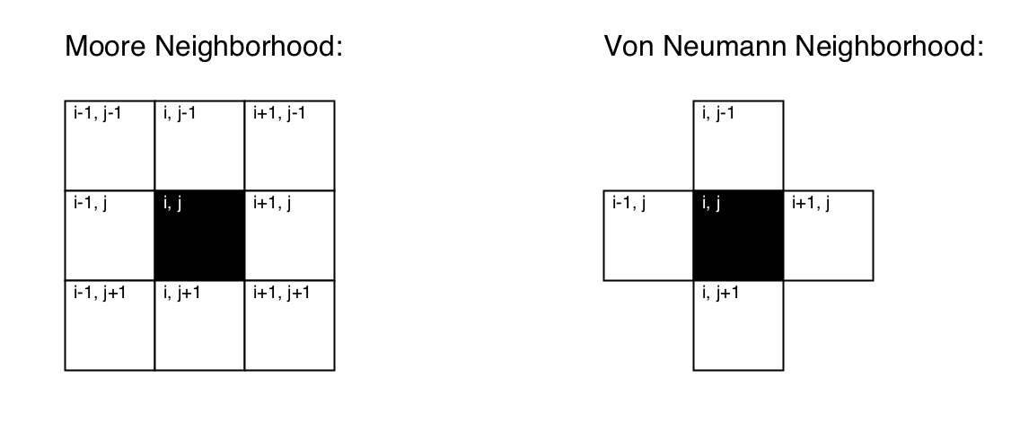
Through the 2 dimensional array it is possible to store now values or objects in different positions of a 2 dimensional grid. In the introductory paragraph it was mentioned that a CA will change its states depending of the states of its neighbours. But how would a cell check these states? the array makes it very easy to find out the indexes of the neighbours of a cell, by checking the cells immediately bellow, above, left and write. There are also different forms of defining which cells one may consider as neighbours. Two typical patterns are the von Neumann and the Moore neighbourhoods:
There are an number of ways of writing code to check the neighbours of a given element in an array. Most of the code in these tutorials uses the Moore neighbourhood; here is a function that sums the values of the Moore neighbours of an element in an array of floats:
float sumNeighbours(float[][] cells, int x, int y){
 float sum=0;
  for(int i=x-1; i<=x+1;i++){
    for(int j=y-1; j<=y+1;j++){
      //if i and j are x and y then it is the cell we are checking,
      //not a neighbour.
      if(i==x && j==y){
      //Continue is a way of making the program skip the
      //rest of the code in the loop where it is called from;
        continue;
      }
      sum+=cells[i][j];
    }
  }
  //it has checked all the neighbours
  return sum;
}
The problems with the edges of the array.
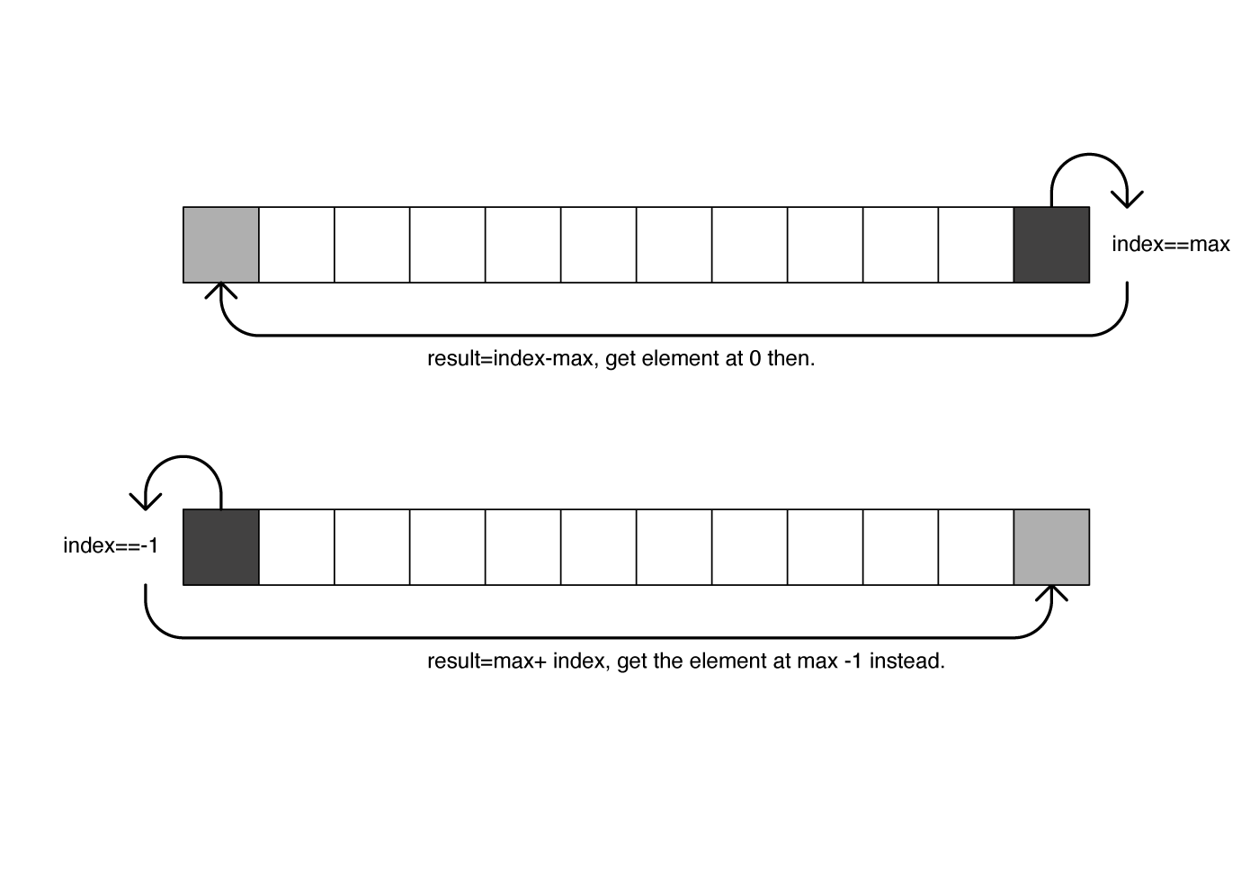
The neighbourhoods above work fine as long as there are always neighbours around the given element; but if the element is on an edge, for example if one of its indices is 0 or if they are on the last column or last row, then the code will produce an ArrayIndexOutOfBoundsException error. A common way to deal with this problem, and to make the CA independent of the effects of having borders or limits, is to wrap the array, similarly to how it was done in the previous tutorial when the coordinates of the agents were wrapped to the size of the display . The function below is an example of how to wrap the cells of a cellular automata, represented in an array. It checks if an index is refers to the left or to the right of the bounds for a given array size (or bottom or top, depending if the test deals with column or row numbers); if it is to the right of the bounds (larger than maxBound) then it returns a corresponding index from the left; it is to the left of the bounds (the index is smaller than 0) it returns an index to the right:
int wrap(int index,int maxBound){
  int result;

  //if it is smaller than 0, return a corresponding value to the left of (smaller than) maxBound
  if(index<0){
     result=maxBound+index;
  }
  //if it is larger than maxBound, return a value at the beginning
  else if(index>=maxBound){
    result=index-maxBound;
  }
  //if the value was valid, then just return it.
  else{
    result=index;
  }
  return result;
}
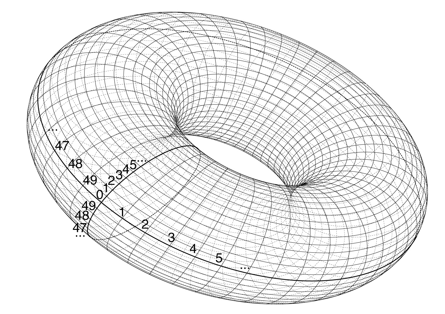
If one considers the effect of this code it will mean that the cells on the leftmost column will have as their neighbours the ones at the rightmost, and vice versa; the same will happen to the cells at the top and bottom rows.If the array would be a sheet of paper, and one could bend it to match this, the result would a torus, like this:
Then and now: arrays and time.
We have seen so far the basic functioning of the neighbourhood of a cell in a cellular automata. As it has been explained, each cell looks at some states of its neighbours and depending of these it changes its own state according to some rules. If we would change the current state of cells depending on the current state of its neighbours, we won’t know what state this cell had when in it is itself the neighbour of another cell. To avoid this we need to somehow store somewhere the new values we are calculating for each cell, and then update them, so the future values become current, and then we can start the process all over.
The code below implements a cellular automata using these techniques. The code is divided in separate parts as small as possible in order to make it modular and easier to debug and understand. A good practice in reading code is to begin from the parts easy to understand and untangle it from there. A typical way of doing this with a Processing program would be to look at the setup() and the draw() functions or methods, and follow the variables and functions initialised and called from there.
The program begins by declaring the 2D array of booleans for the current states, and another 2D array to store the future states. We also use a couple of variables to define the size of the arrays, and the size in pixels of each cell:
boolean[][] cellsNow; //2 dimensional array of booleans
boolean[][] cellsFuture; //2 dimensional array of booleans
int columns, rows;
int scale=5; //this means that the cells will be 5x5 pixels...
Now we go to the setup():
void setup(){

size(500,500);

frameRate(1); //one frame per second...slow motion
background(255); //draw background white
//stroke for showing the cells
stroke(200);
strokeWeight(0.5);

//we calculate the number of columns and rows so they fill the screen
//when we draw them...
columns=width/scale;
rows=height/scale;

cellsNow=new boolean[columns][rows]; //in an array, booleans will be automatically set to false...
cellsFuture=new boolean[columns][rows];

//we set the cell at the centre "on" (true)
cellsNow[columns/2][rows/2]=true;

}
So far everything looks quite similar to the previous example…We also have a draw:
void draw(){
  background(255); //clean the background
  drawCells(); //call function drawCells, described below

  tick(); //calculate future values (below)
  update(); //another function below
}
That calls first a “drawCells();” function, which includes a nested loop:
void drawCells(){
  for(int i=0;i<columns;i++){//we go through all the columns
    for(int j=0;j<rows;j++){
      if(cellsNow[i][j]==true){
        fill(0); //black if true
      }else{
        fill(255); //white if false
      }
      rect(i*scale,j*scale,scale,scale);
    }
  }
}
And two other functions: one called “tick()” (as the tick of a clock), and which simply calculates the future values, and another called “update()”. This is the “tick()” function:
void tick(){
  for(int i=0;i<columns;i++){//we go through all the columns
    for(int j=0;j<rows;j++){
      int numNeigs= countNeighbours(i,j);
       cellsFuture[i][j]=applyRules(numNeigs);
    }
  }
}
It iterates through all cells with a nested loop, as we have seen, and it calls two other functions: “countNeighbours()”, which takes i and j as parameters, and which returns and sets an int variable called numNeigs; we then use “applyRules()”, to set the future state of each cell. We will look first at countNeighbours(), which also calls the helper function “wrap()”, which we have already defined:
int countNeighbours(int col,int row){
  //this is what is generally known as the "Moore neighborhood".
  //it comprises the 8 cells surrounding the one in col and row.
  //We have to be carefull with the cells in the borders (col==0,
  //col==colums-1, row==0 and row==rows-1). We decide to use a method
  //similar to the"wrap around world" we have seen with the particles/agents.

  int totalNeighbours=0;

  for(int i=col-1;i<=col+1;i++){
    //wrap the column.
    int neigColumn=wrap(i,columns);
    for(int j=row-1;j<=row+1;j++){
      //wrap the row.
      int neigRow=wrap(j,rows);
      // if this neighbour is "on" (true) we add it
      if(cellsNow[neigColumn][neigRow]==true){
        totalNeighbours++;
      }
    } //end of row loop
  } //end of column loop

  return totalNeighbours;
}

//this is the wrap function, as explained above.
int wrap(int index,int maxBound){
  int result;
  if(index<0){
     result=maxBound+index;
  }
  else if(index>=maxBound){
    result=index-maxBound;
  }
  else{
    result=index;
  }
  return result;
}
Now that we have seen what “countNeighbours()” does, lets see what the other function called from “tick()”, that is, “applyRules()” does:
boolean applyRules(int numNeigs){

  boolean[] rules=new boolean[10];
  rules[0]=false;
  rules[1]=true;
  rules[2]=true;
  rules[3]=true;
  rules[4]=false;
  rules[5]=false;
  rules[6]=false;
  rules[7]=false;
  rules[8]=true;
  rules[9]=false;

  return rules[numNeigs]; //depending of the number of neighbours it will return a value
}
this is a way of using rules depending of the neighbours, and it actually does not need a function (it would have been possible to declare the rules somewhere and just use them as in the function). Using a function, in the other hand, makes it easy to modify. The number of neighbours may range from 0 to 9 (if we count the current cell), so one can use an array to store the results of each of the possible cases. This is sometimes called a “look up table”. There are other ways of implementing the rules, for example with a few if() or with a switch() statement, a convenient way of writing a piece of code that does different things depending of the values of a variable, instead of using many if() and if else() statements.
Finally the “update()” function; it just copies the values calculated for the future as present, that is, all values from the cellsFuture array to the cellsNow array:
void update(){
  //copying all values.
  for(int i=0;i<columns;i++){//we go through all the columns
    for(int j=0;j<rows;j++){
      cellsNow[i][j]=cellsFuture[i][j];
    }
  }
}
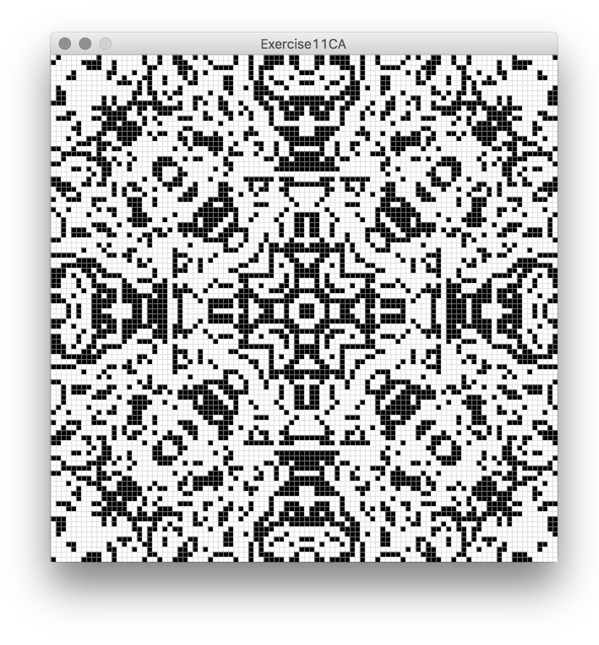
There is a more efficient ways of doing this with what is known as a “swap” which makes use of references. Next tutorials and examples will use that method instead, but but to reduce the amount of new concepts introduced, the code above uses direct copies. Here is the result after a few iterations:
Although the code is quite long, most of it is made of similar and repeated parts such as the nested loops. The logic of the Cellular automata is also quite simple. Here is a link to a processing file with the code: Exercise11CA
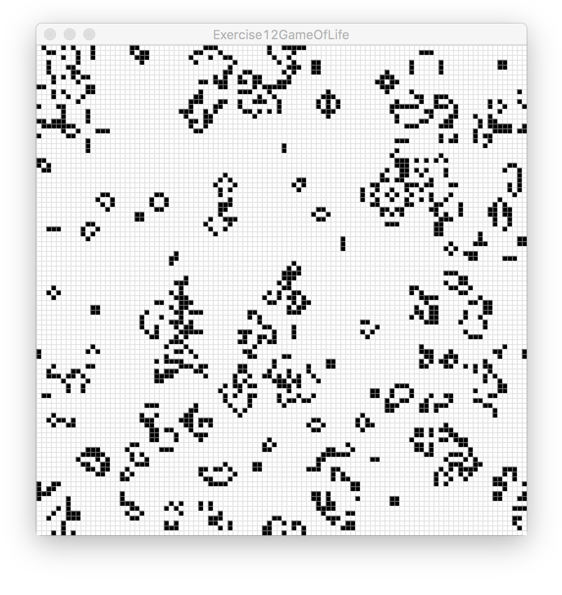
This Cellular automata is loosely based in the rules described by Stephen Wolfram in “a New Kind of Science”, in Chapter 5, “Two Dimensions and Beyond”. You can try different rules and study the basics of the cellular automata. Study the references and links given, particularly other CA code written in Processing, see how it differs from the one presented here. You can for example look at one of the most famous CAs, Conway’s “Game of Life”, see the rules and think how you could implement it. The only necessary thing to do is to modify the applyRules() function, so it can also consider the current state of the cell (if it is alive or dead) and apply the specific rules of the “Game of Life”. Also the initial conditions will need to be modified in the setup(), so one can see something interesting happening. Here is the modified version of the CA program: Exercise12GameOfLife
