Fifth Tutorial: putting everything together.
Everything together.
The following tutorial will look at how to take the models used in early tutorials from 2D to 3D. It will also introduce a library developed for the course that makes easier to output voxel 3D data.
Three dimensional Cellular Automata.
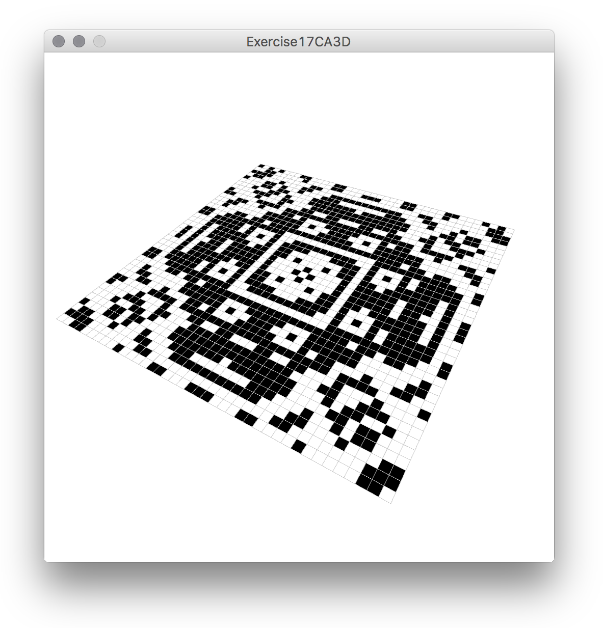
Now it is possible to modify the Cellular Automata code to draw it in 3D, by adding PeasyCam and changing it slightly, to produce this:
Here is the modified code. All 2D drawing operations work still on 3D. But even if one can rotate it i 3D, it is obviously a 2D CA. One could render it with solids or boxes, but it would not make much of a difference. There are a number of options to use 3D dimensions. for example, it is possible to write a CA that instead of checking its 8 2D neighbours of the Moore neighbourhood (or 4 of the von Neumann… see the third tutorial) checks instead 3dimensional 26 neighbours, in a 3Dimensional lattice. Another possibility is to use the third dimension to store the history of the 2D CA, like Wolfram does in A New Kind of Science, which is what the following example does. There are a number of other interesting examples of 3Dimensional cellular automata in A New Kind of Science.
The 2D Cellular Automata then needs to be modified like this: it needs a 3D array to store its history, declared as follows:
//this is a 3dimensional array used to store the history of the CA
boolean[][][] history;
int historyLength=60; //the maximum amount of CA steps to store
int currentTime=0;
which will be created in setup() and will have the same width and height as the 2D CA:
//these are the same as previously:
cellsNow=new boolean[columns][rows];
cellsFuture=new boolean[columns][rows];
//this is the new history 3D array:
history=new boolean[columns][rows][historyLength];
for storing the values in history, we will call a function like this one every time we update the CA:
void recordHistory(){
 //to prevent storing beyond the capacity of history
 if(currentTime>=historyLength){
   return;
 }
 //if it reaches here, currentTime is smaller than historyLength.
 //so we have not exceeded the capacity of the history array

//store the current states in history, at currentTime
 for(int i=0;i<columns;i++){//we go through all the columns
   for(int j=0;j<rows;j++){ //all the rows
     history[i][j][currentTime]=cellsNow[i][j];  //and copy them into history
   }
 }
 currentTime++; //increase current time, so next time we write on the layer on top
}
And instead of drawing the 2D CA, the sketch will draw now the history, like this:
void drawHistory(){
 for(int i=0;i<columns;i++){//we go through all the columns
   for(int j=0;j<rows;j++){ //and all the rows...
     //and all the layers of history, from 0 to currentTime
     for(int k=0;k<currentTime;k++){
       if(history[i][j][k]==true){ //draw only if true
         pushMatrix(); //we store the current transformations
         translate(i*scale,j*scale,k*scale); move to a position to draw
         //sphere(scale/1.5); //one could draw spheres, instead
         box(scale,scale,scale); //...but we draw a box
         popMatrix(); // restore transformations.
       }
     }
   }
 }
}
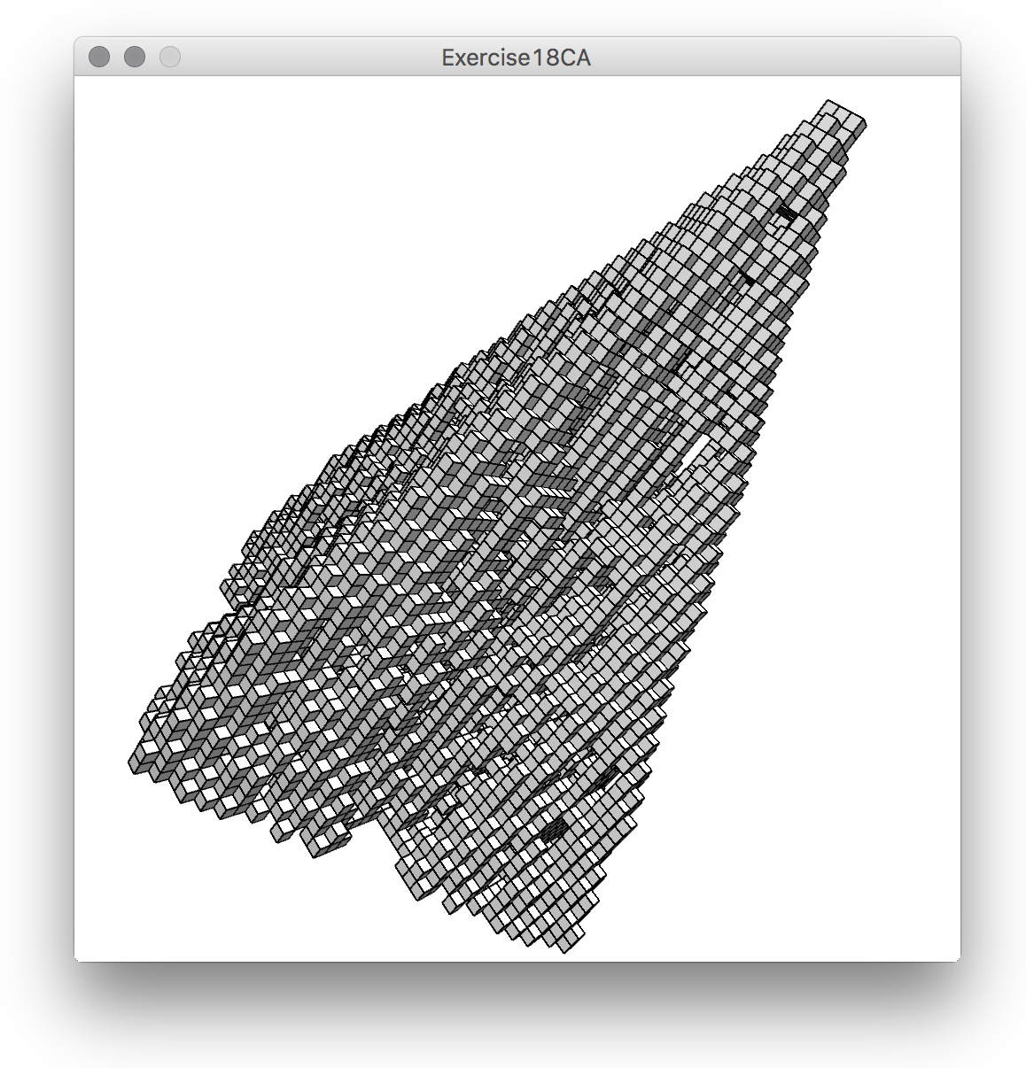
This should work fine now… but actually while the 2D CA above looks quite nice in 2D it is a bit dull in 3D, so following are a few modifications of the CA to make it look a bit more interesting. What these do is to make it identical to the 2D CAs in A New Kind of Science, specially those in page 177 and onwards. In the first place we change the applyRules() function that we defined in the first CA to something like this:
boolean applyRules(boolean me, int numNeigs){
 if(me==true){
   return trueRules[numNeigs];
 }else {
   return falseRules[numNeigs];
 }
}
And we define the rules somewhere else, for example in the beginning of the sketch, like this:
//Wolfram rule 746
boolean[] trueRules={
	true,
	true,
	true,
	true,
	true,
	false,
	false,
	false,
	false,
	false,
};
boolean[] falseRules={
	false,
	false,
	false,
	true,
	false,
	false,
	false,
	false,
	false,
	false,
};
This is, by the way, another syntax for initialising arrays, if one knows what values it is going to have from the beginning… it is just easier than having to write
trueRules=new boolean[10];
trueRules[0]=true;
trueRules[1]=true;
trueRules[2]=true;
//...etc
inside setup(). There are also a couple of modifications to the countNeighbours(), so it only counts the number of neighbours that are on, and exclude the state of the cell at the centre. Also, in the initialisation in setup() we turns 3 contiguous cells on, instead of only one. Other small changes include some code for the lighting in draw(). Here is all the code with modifications:
import peasy.*;
PeasyCam cam;

boolean[][] cellsNow; //2 dimensional array of bools
boolean[][] cellsFuture; //2 dimensional array of bools

boolean[][][] history; //this is a 3dimensional array used to store the history of the CA
int historyLength=60; //the maximum amount of steps to store
int currentTime=0;

int columns, rows;
int scale=5;

//Wolfram rule 746
boolean[] trueRules={
  true,
  true,
  true,
  true,
  true,
  false,
  false,
  false,
  false,
  false,
};
boolean[] falseRules={
  false,
  false,
  false,
  true,
  false,
  false,
  false,
  false,
  false,
  false,
};

void setup(){

size(500,500, P3D);
pixelDensity(displayDensity());
cam = new PeasyCam(this, 400);
background(255); //draw background white
columns=80;
rows=80;

cellsNow=new boolean[columns][rows];
cellsFuture=new boolean[columns][rows];
history=new boolean[columns][rows][historyLength];

//this sets a row of 3 contiguous cells at the centre as true
cellsNow[columns/2][rows/2]=true;
cellsNow[columns/2][rows/2-1]=true;
cellsNow[columns/2][rows/2+1]=true;
}

void draw(){

  background(255); //clean the background

  //set some lighting...
  ambientLight(30,30,30);
  lightSpecular(255,255,255);
  directionalLight(255,255,255,-30,60,-50);

  //to center the CA and make it look nice at the start
  rotateY(-2*PI/3);
  rotateX(-PI/3);
  translate(-scale*columns/2,-scale*rows/2,-scale*historyLength/2);

  drawHistory(); //draw
  tick(); //calculate future values
  recordHistory();
  update();
}

void drawHistory(){
  for(int i=0;i<columns;i++){
    for(int j=0;j<rows;j++){
      for(int k=0;k<currentTime;k++){ //we go through all previous states
        if(history[i][j][k]==true){ //draw only if true
          pushMatrix();
          translate(i*scale,j*scale,k*scale);
          //sphere(scale/1.5);
          box(scale,scale,scale);
          popMatrix(); //needs to be called eventually after pushMatrix().
        }
      }
    }
  }
}

void tick(){
  for(int i=0;i<columns;i++){
    for(int j=0;j<rows;j++){
      int numNeigs= countNeighbours(i,j);
       cellsFuture[i][j]=applyRules(cellsNow[i][j],numNeigs);
    }
  }
}

int countNeighbours(int col,int row){

  int totalNeighbours=0;
  for(int i=col-1;i<=col+1;i++){
    //wrap the column.
    int neigColumn=wrap(i,columns);
    for(int j=row-1;j<=row+1;j++){
      //wrap the row.
      int neigRow=wrap(j,rows);
      //now we only count the neighbours, excluding the cell at the centre.
      //if either the column or the row we are looking at are different that col
      //and row, we know it is not the cell at the centre.
      if(neigColumn != col || neigRow != row){
        // if this neighbour is "on" (true) we add it
        if(cellsNow[neigColumn][neigRow]==true){
          totalNeighbours++;
        }
      }
    } //end of row loop
  } //end of column loop
  return totalNeighbours;

}

//this is the wrap function.
int wrap(int index,int maxBound){
  int result;
  if(index<0){ result=maxBound+index; } else if(index>=maxBound){
    result=index-maxBound;
  }
  else{
    result=index;
  }
  return result;
}

boolean applyRules(boolean me, int numNeigs){
  if(me==true){
    return trueRules[numNeigs];
  }else {
    return falseRules[numNeigs];
  }
}

void update(){
  //copying all values.
  for(int i=0;i<columns;i++){
    for(int j=0;j<rows;j++){
      cellsNow[i][j]=cellsFuture[i][j];
    }
  }
}

void recordHistory(){
  //to prevent storing beyond the capacity of history
  if(currentTime>=historyLength){
    return;
  }
  //if it reaches here, currentTime is smaller than historyLength.

  //store the current states in history, at currentTime
  for(int i=0;i<columns;i++){
    for(int j=0;j<rows;j++){
      history[i][j][currentTime]=cellsNow[i][j];
    }
  }
  currentTime++; //increase current time
}
And this is the result:
Here is the code in a zip file.
For anyone interested in experimenting with more of Wolfram rules, this is a little bit of code that will generate rules that can be used in the code above from his numbering system. Basically what Wolfram does is to encode all the trues and false of the tables as ones and zeros of a binary number. For example, the rule used in the code above would be 000001111 and 000000100; interlaced, as Wolfram does, it would become 000000000010111010, a binary number that in decimal is 746. This is a complicated encoding for beginners, so the simple sketch below translates a decimal number into the rules using something called bitwise operators (also a bit esoteric and not generally used in programming with Processing). The code is handy if anyone wants to translate the rules from A New Kind of Science into rules that the CA above can use:
boolean[] trueRules=new boolean[10];
boolean[] falseRules=new boolean[10];

void setup(){
  makeRulesFromWolfram(764);
}


void makeRulesFromWolfram(int rule){ //generate rules from Wolfram encoding
  for(int i=0;i<10;i++){
    falseRules[i] = (rule & 1<<(2*i))!=0;
    trueRules[i]  = (rule & 1<<(2*i+1))!=0;
  }
  println("//Wolfram rule "+rule);
  println("boolean[] trueRules={");
  for(int i=0;i<10;i++){
    println("\t"+trueRules[i] +",");
  }
  println("};");
  println("boolean[] falseRules={");
  for(int i=0;i<10;i++){
    println("\t"+falseRules[i] +",");
  }
  println("};");
}
This code generates a text that is formatted so it can be copy-pasted onto the code of the CA above. Of course, another solution is to simply include the code directly into the sketch, and call it in the setup() with the number of the rule we want to generate.
To export the geometry from the program above one could use the dxf library as in the previous tutorial, or other library that can output 3D data. This however may turn out to be not as straightforward as it may seem. As part of this course we have developed a library for visualising and exporting voxel data (like the one used by the CA above) as .stl files. Stl files can be either directly 3D printed or they can also be imported into many CAD and modelling software. To install the library just follow the instructions here. (there is also a link under “resources”, to the right on this page).
The CA above can be easily modified once more to make use of this voxel library, and in fact simplify its drawing. It is necessary first to import it in the code, either through “Sketch->Import Library->Voxel Library” or by writing directly
import voxellib.*;
We need then to declare a Mesh object:
Mesh mesh; //from our very own voxellib
and create it in setup(), like this:
mesh=new Mesh(this);
Now we can use it in draw(). Instead of using the drawHistory() method that the code above uses, we can delete it and use instead
mesh.makeFromVoxels(history,scale); //to update the mesh
 mesh.draw(); //to draw the mesh
For saving it as an .stl file (in the sketch’s folder) one only needs to write:
mesh.saveAsStl("someNameForTheFile.stl");
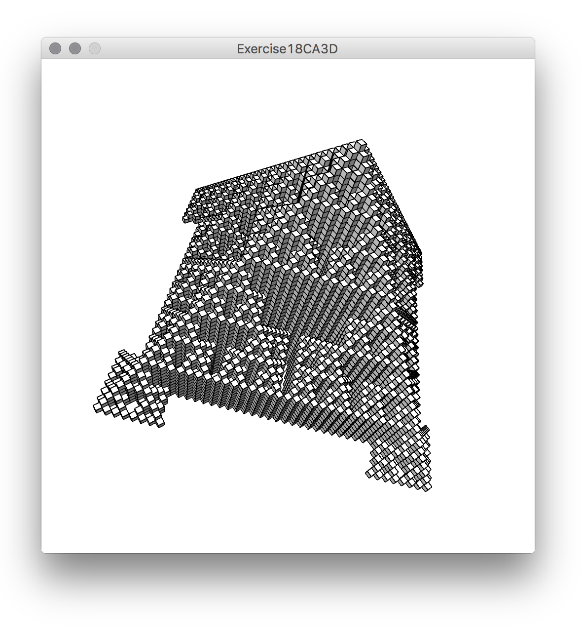
Here is the code for an updated version of the CA, using the Voxel Library. Besides being able to save as .stl, the big difference of the library is how it draws the 3dimensional pixels or voxels: instead of drawing many cubes, it just draws the walls between solid and empty, or true and false cells. This means that, since it skips all walls between cubes lying beside each other, it has less walls to draw and it renders faster. A problem that may arise from the .stl file is that, since the edges of the cubes touch each other, they generate what is called “manifold meshes” (if the .stl file is loaded in a CAD package, the program may flag it up). However, this is not generally a problem for inkjet based 3D printers.
Before moving on, bellow is a version of similar cellular automata to the one we have just looked at, also using the Voxel Library. In this case the CA uses the von Neumann neighbourhood (as explained in the third tutorial), and implements the rules also from A New Kind of Science. The encoding of the rules is similar, and in this case the sketch includes the function to decode them from Wolfram’s condensed (but cryptic) encoding.
The code can be downloaded here.
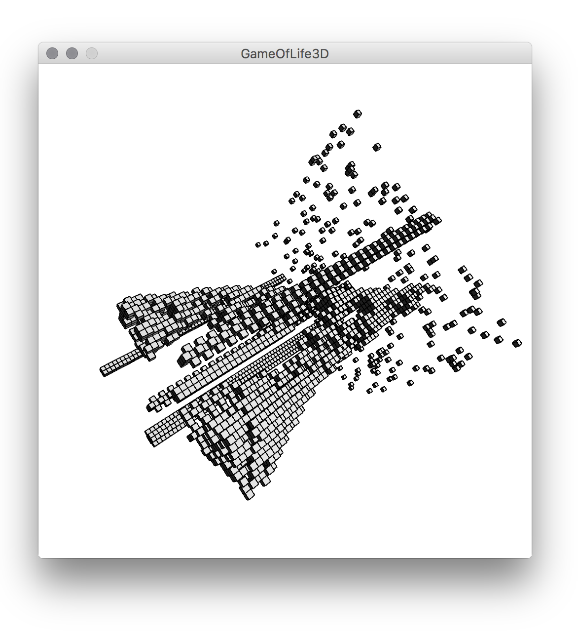
And finally, if anyone wants to see what happens with a 3Dimensional Game of Life, here it is:
And here is the code: GameOfLife3D
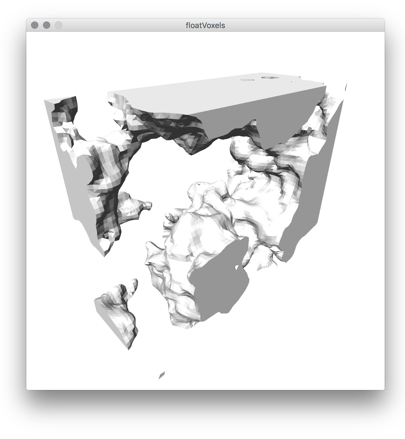
But the Voxel Library cannot only take boolean voxels (or 3D pixels), it also accepts float voxels. The program called floatVoxels.pde is one of the examples included with the library; it uses Perlin noise through the Processing function noise() to create a smooth but random distribution of values within the voxels, and then wraps what is called an isosurface. An Isosurface is the 3D equivalent of an isoline or a contour line, typical of topographic maps or weather maps. The method used to calculate this iso surface is known as the Marching cubes algorithm, which is used to generate 3D solid from medical CT or MRI data, for example. This is the result of running the floatVoxel.pde example:
Now it is possible to revisit some of the particles we used and make them in 3D, and somehow let them modify the voxels. Lets start with the particles, and make them into 3D; a minimal code would look something like this (using PVector, which, although a bit complicated it actually makes live easier in 3D):
import peasy.*;
PeasyCam cam;

int numParticles=1000;
PVector particlePos[]; //the position of the particles as PVectors
PVector particleDir[]; //the direction of the particles as PVectors

void setup(){
 size(500,500, P3D);
 pixelDensity(displayDensity());
 cam = new PeasyCam(this, 400);

 //now we create the particles
 particlePos=new PVector[numParticles];
 particleDir=new PVector[numParticles];

 for(int i=0;i<numParticles;i++){
   //a random position and direction
   // it creates a random position, but only one unit distance from the origin
   particlePos[i]=PVector.random3D();
   particleDir[i]=PVector.random3D();
 }

}

void draw(){

 background(255);

 for(int i=0;i<numParticles;i++){
   //this is a bit of a complicated way of writing the PVector
   //stuff...it just adds the current direction of the
   //particle multiplied by 0.05. If we would not do the .copy() before mult()
   //we would multiply the particleDir[i], so it would get smaller and smaller
   //every time, as we would be multiplying it by 0.05.
   //the line can be read then as "add to particlePos[i] a copy of particleDir[i]
   //multiplied by 0.05".
   particlePos[i].add(particleDir[i].copy().mult(0.05));
   //wiggle a bit...
   particleDir[i].add(PVector.random3D().mult(0.05));
 }

 //draw the particles
 strokeWeight(10);
 for(int i=0;i<particlePos.length;++i){
   point(particlePos[i].x,particlePos[i].y,particlePos[i].z);
 }

}
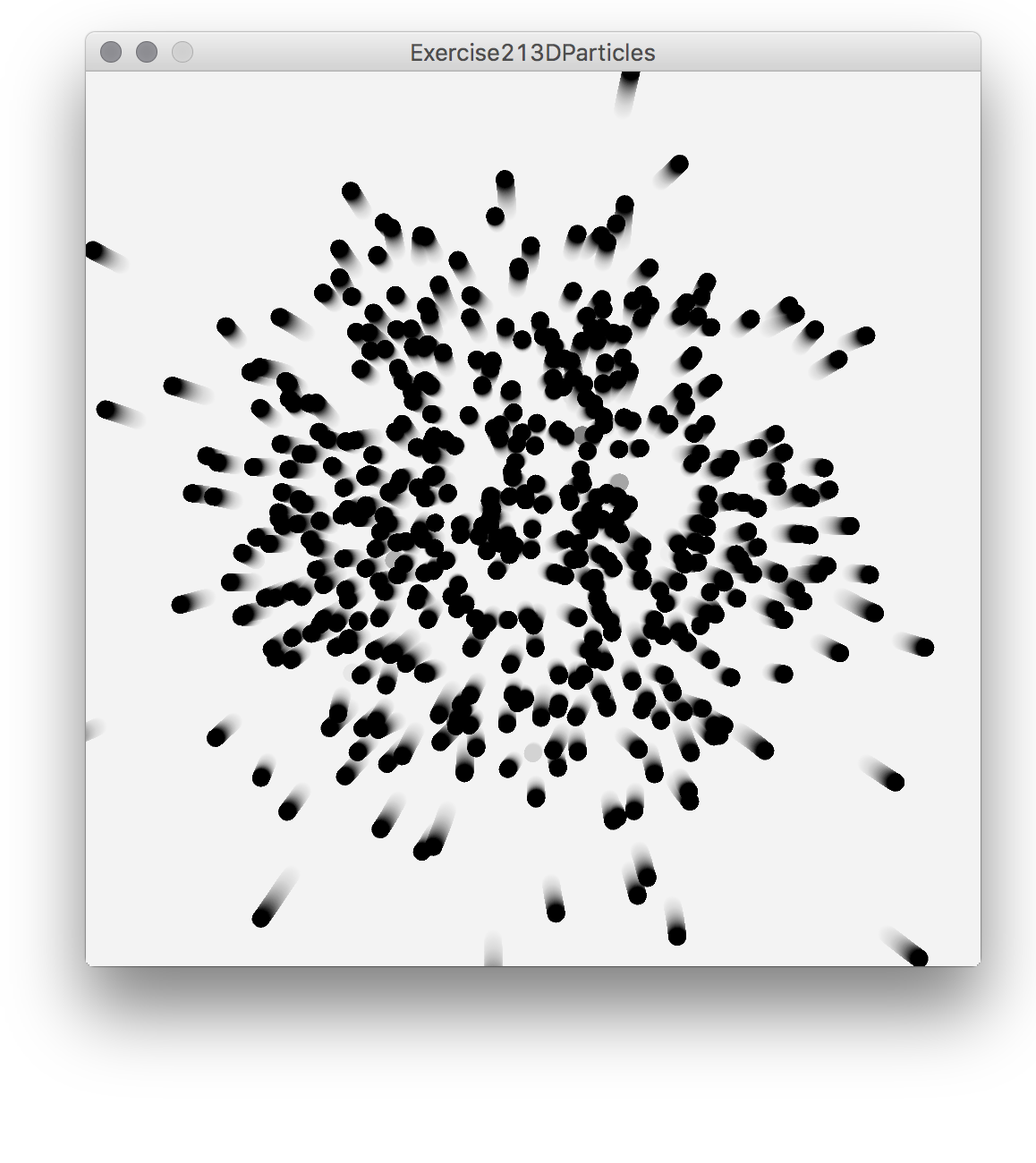
Which would result in something like this (rendered with a bit of motion blur…):
Now we have to make them leave traces on voxels, and use the Voxel Library to render and export the 3D data. The idea then is how to make them interact with the voxels? if one imagines that the particles move through a 3D grid representing the voxels, to know the indices of the voxels they are in, we would need to simple to divide the x,y and z of the particle by the size of the boxels, and then make that number into an integer. something like this:
for(int i=0;i<numParticles;i++){
 int voxelX=int(particlePos[i].x/voxelSize);
 int voxelY=int(particlePos[i].y/voxelSize);
 int voxelZ=int(particlePos[i].z/voxelSize);
 }
Because in the code we are going to assume a size of the each voxel of 1 (it makes life easier), in order to know in which voxel they particles are we only need to convert their coordinates into integers. Because we are going to use these numbers as indices for an array, we also need to make sure that they are within the range of the indices of the array (not negative, or otherwise larger than the sizes of the array, which would then refer to inexistent cells). This is the resulting code:
import peasy.*;
import voxellib.*;
PeasyCam cam;
Mesh mesh;

int numParticles=2000;
PVector particlePos[];
PVector particleDir[];

int sizeX=50;
int sizeY=50;
int sizeZ=50;

float[][][] voxels;

void setup(){
 size(500,500, P3D);
 pixelDensity(displayDensity());
 cam = new PeasyCam(this, 400);

 mesh=new Mesh(this);

 //create the voxels
 voxels=new float[sizeX][sizeY][sizeZ];

 //create the particles
 particlePos=new PVector[numParticles];
 particleDir=new PVector[numParticles];

 for(int i=0;i<numParticles;i++){
   //a random position and direction
   // it creates a random position, but only one unit distance from the origin
   particlePos[i]=PVector.random3D();
   particleDir[i]=PVector.random3D();
 }

}

void draw(){
 background(255);
 //set some lighting...
 ambientLight(30,30,30);
 lightSpecular(255,255,255);
 directionalLight(255,255,255,-30,60,-50);

 for(int i=0;i<numParticles;i++){
   particlePos[i].add(particleDir[i].copy().mult(0.05));
   //wiggle a bit...
   particleDir[i].add(PVector.random3D().mult(0.05));
 }

 for(int i=0;i<numParticles;i++){
   int voxelX=int(particlePos[i].x);
   int voxelY=int(particlePos[i].y);
   int voxelZ=int(particlePos[i].z);
   //these are the conditions that make sure that the positions are valid indices
   //for the array. Instead of writing many ifs it just uses lots of && (AND)
   if(voxelX>=0 && voxelX<sizeX &&
      voxelY>=0 && voxelY<sizeY &&
      voxelZ>=0 && voxelZ<sizeZ) {
      voxels[voxelX][voxelY][voxelZ]+=0.1;
   }
 }

 //draw the particles
 strokeWeight(2);
 for(int i=0;i<particlePos.length;++i){
   point(particlePos[i].x,particlePos[i].y,particlePos[i].z);
 }

 noStroke();
 //update and draw the mesh. We pass first the size of each voxel (1.0 in this case)
 //and the level to draw. 0.5 will create a surface between values larger than 0.5
 //and smaller than 0.5.
 mesh.makeFromVoxels(voxels,1,0.5f);
 mesh.draw();
}
Observe also the call to the Voxel Library function. It specifies the size (1,0) of the voxels first, and the level, which is 0.5 in this case. Think of the level as the 3D equivalent to the height of the iso curve in a topographic map: it defines the boundary between values larger and smaller than the level:
mesh.makeFromVoxels(voxels,1,0.5f);
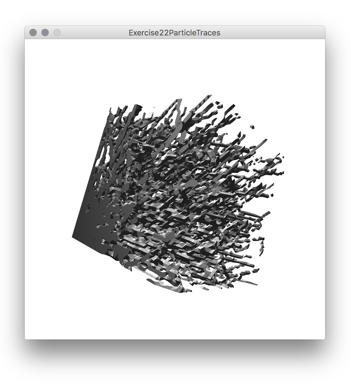
And the result looks something like this:
It is ok, but not that terribly exciting. To make it look a bit nicer, instead of leaving a trace only in the single voxel that the particle finds itself at a certain moment, we can make it leave a trace also on the surrounding voxels, a smaller quantity the further these “traced” cells are from the particle. A function of distance that produces nice results is the Gaussian function. It is the same mathematical function used in for example gaussian filters in image processing. Below is the code to leave a Gaussian trace on voxels from a given position. The functions takes a PVector with the position and the radius we want to affect (if it is smaller than one it will only affect the closest cell).
void stampGaussian(PVector pos, float radius){

  int xPos=int(pos.x);
  int yPos=int(pos.y);
  int zPos=int(pos.z);

  int rad=int(radius)+1;

  //iterate through all the voxels that are within the given radius
  for(int x=xPos-rad; x<=xPos+rad ; x++) {
   for(int y=yPos-rad; y<=yPos+rad ; y++){
     for(int z=zPos-rad; z<=zPos+rad ; z++){ //if valid, calculate the distance and the Gaussian function if(x>=0 && x=0 && y=0 && z<sizeZ){

          float distance=PVector.dist(new PVector(x,y,z), pos);
          //the Gaussian function
          float a=radius/2; //this is the range for the Gaussian function
          float b=5;
          float func=b*exp(-distance*distance/(2*a*a)); //this is the Gaussian function
          voxels[x][y][z] += 0.01* func;
        }

      }
    }
  }
}
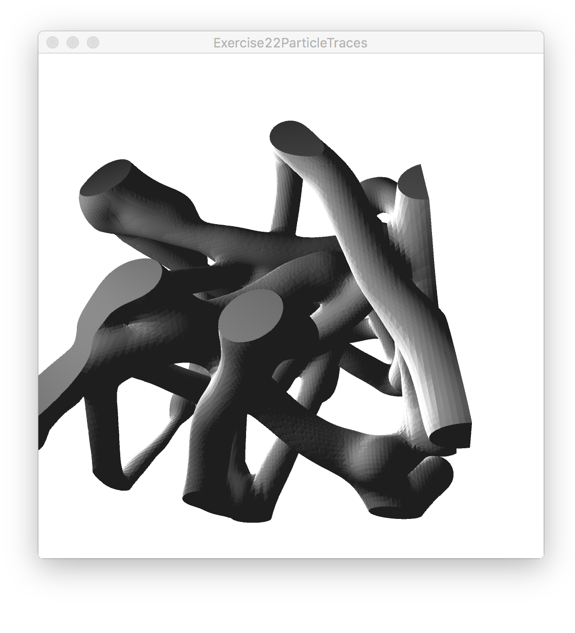
Besides this, we can also make the particles bounce on the limits of the space defined by the voxels and make them start at random points within the voxels. After this and other tweaks, this is the result:
Here s the code all the code together: Exercise22ParticleTraces
Basically this covers all what there is to learn in the course…
